What is Part Average Testing PAT?
Hidden reliability issues in ICs often remain undetected during production, only to appear once the chip is in use, potentially leading to costly system disruptions.
What if you could harness the massive data from semiconductor testers to uncover insights that help you catch issues early—preventing costly retests and failed dies down the line?
The semiconductor industry addresses this challenge through Part Average Testing (PAT), a powerful outlier detection method that screens each die and sets limits across multiple test parameters. Any die outside these statistically determined limits is flagged as an “outlier,” allowing manufacturers to catch defects early and maintain higher yield quality.
Each IC design and its unique processing flow create distinct test result statistical distributions which become the foundation for setting PAT limits. Automotive engineers have applied PAT to electrical test measurements for nearly three decades, making it a mainstay in achieving rigorous standards.
In this blog, you’ll learn the foundational aspects of PAT, examine its different types, and the advanced capabilities of the yieldWerx PAT module. We base this discussion on Automotive Electronics Council’s (AEC) guidelines, the globally accepted standard for Part Average Testing. The principles described in this guideline apply to packaged or unpackaged die.
What are the benefits of PAT?

The demand for quality, reliability, and transparency in the semiconductor industry is rising sharply, with zero tolerance for defects becoming the standard—especially in sectors like automotive.
- By providing early feedback on outlier components, PAT helps prevent quality incidents before they escalate, significantly reducing expenses related to customer support and failure analysis.
- This proactive approach leads to a notable decrease in Return Material Authorizations (RMAs) and failure analysis requests from the field.
- PAT contributes to packaging cost savings at the wafer level, as only parts that meet quality standards proceed through more expensive stages of production.
- Automatic bin adjustments within PAT allow for real-time quality indications, providing ongoing assurance of product reliability.
- Through outlier limit optimization, PAT reinforces high-quality standards, ensuring that customers only receive reliable devices.
Investing in Outlier Detection and Part Average Testing (PAT) ensures high quality and reliability, reinforcing your brand’s reputation with customers and their clients.
The outlier detection in the die-level PAT screening can be both static and dynamic.
Ready to optimize your yield? Discover how yieldWerx’s automotive solutions can transform your quality control strategy—get in touch today!
What is Static PAT?
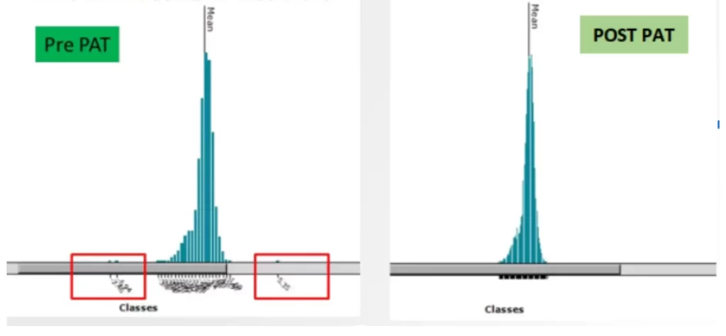
Static PAT (SPAT) sets clear boundaries to catch outliers, using a predefined set of tests and population data from multiple batches. These boundaries—called the lower and upper specification limits (LSL and USL)—act as a guardrail for screening dice that fall outside acceptable ranges. Updated every six months or after eight wafer lots (whichever comes first), SPAT calculates the mean (µ) and standard deviation (σ), setting limits at µ ± 6σ to ensure only quality parts move forward.
Static PAT Limits = Robust Mean ± 6 Robust Sigma
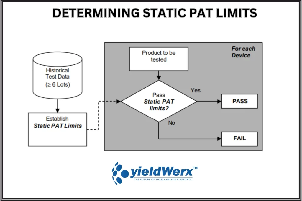
Source: AEC Guidelines
What is Dynamic PAT?
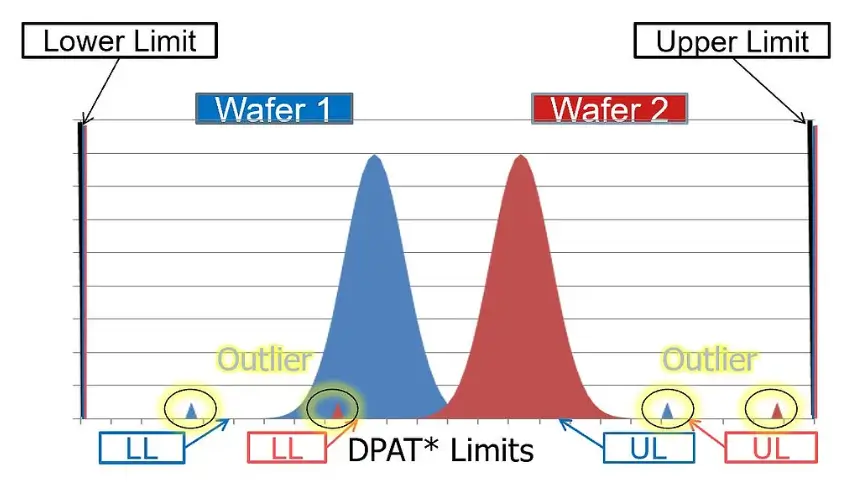
Source: ATE Service JAPAN
SPAT can lead to excessively wide distributions compared to batch-by-batch estimates. Instead, Dynamic PAT (DPAT) takes a real-time approach, setting limits individually for each wafer test by calculating the mean and standard deviation for a specific lot. These limits are based on the actual material in front of you, eliminating lot-to-lot variation concerns.
Here’s the key: any die that falls outside the DPAT limits but remains within broader specification limits (LSL and USL) is flagged as an outlier. Since wafer distributions are often tighter than those of entire lots, DPAT lets you fine-tune limits to each wafer’s unique profile, quickly identifying any deviations from the norm.
Dynamic PAT Limits = Robust Mean ± 6 Robust Sigma
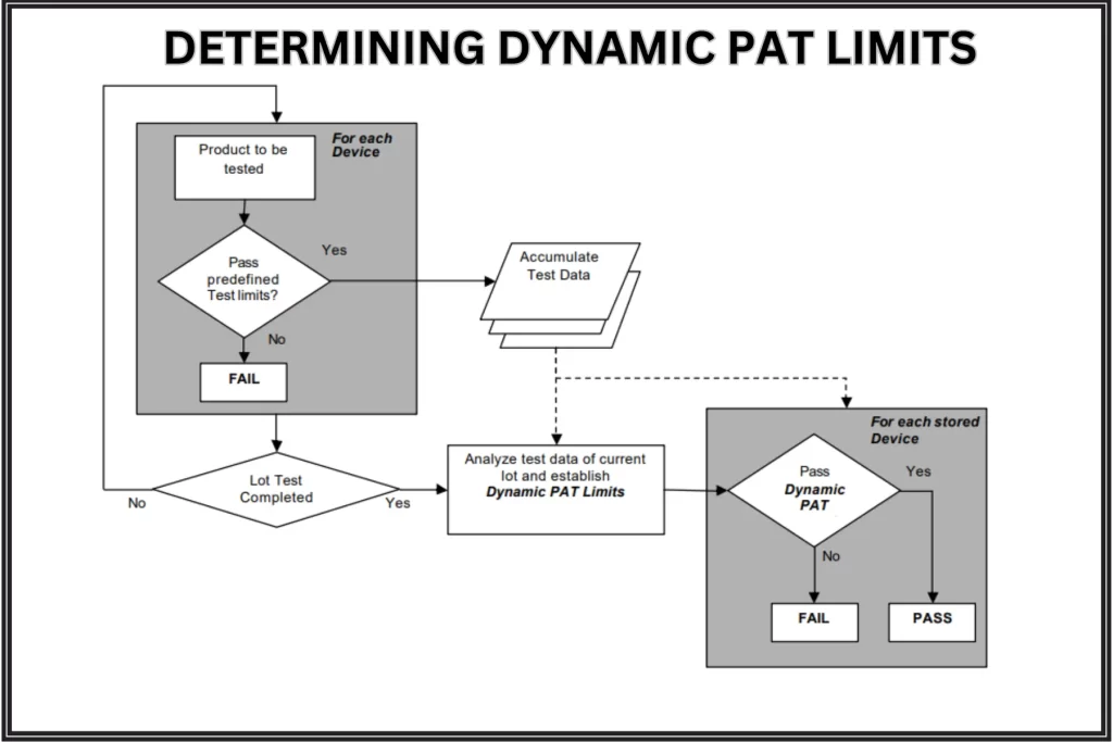
According to a KeySight case study, implementing pseudo-real-time Dynamic PAT limits instead of the per lot Static PAT limits process led to a reduction of greater than 2% in the total false rejects, a reduction of unnecessary scrap, a reduction of device handling, and improved equipment throughput due to the lower retest rate.
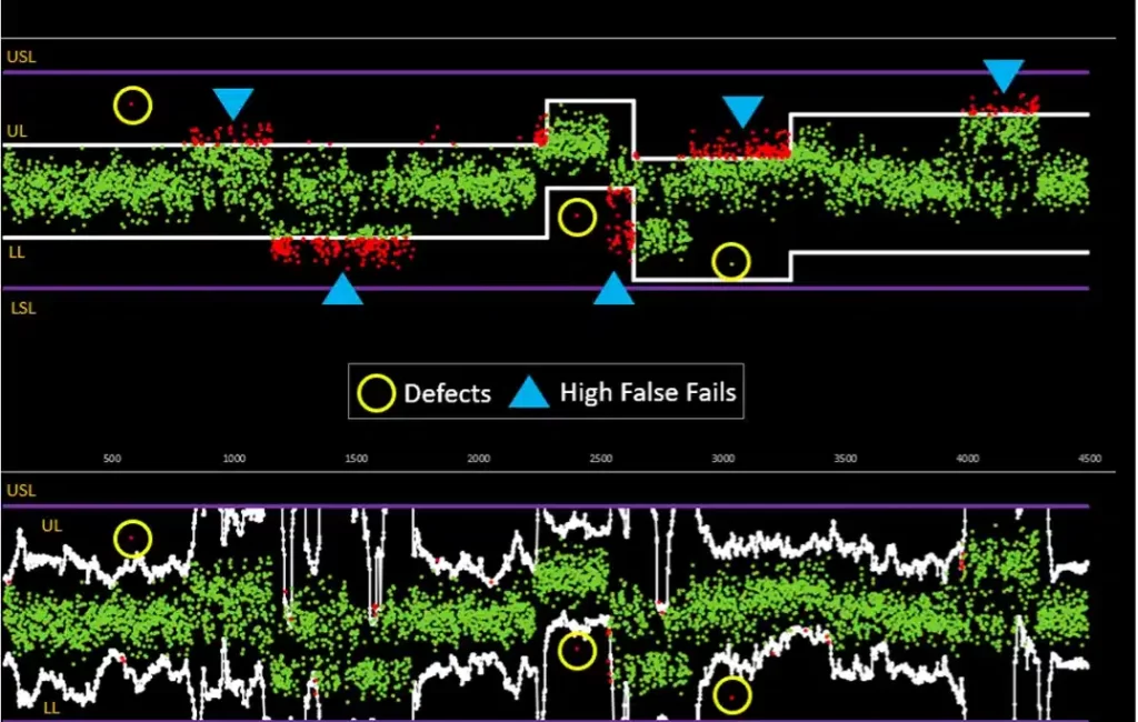
Keysight: Static Vs Dynamic PAT Limits
Setting PAT Limits: Tailoring for Normal vs. Non-Normal Data
PAT for Normal Distribution
Calculating Part Average Testing (PAT) limits differs for normal and non-normal distributions because of the unique characteristics of each. A normal distribution is symmetrical, where data clusters around a central mean, forming a bell-shaped curve with most data points falling within three standard deviations. For such distributions, PAT limits are set using the robust mean and standard deviation method, effectively identifying outliers based on their distance from the mean.
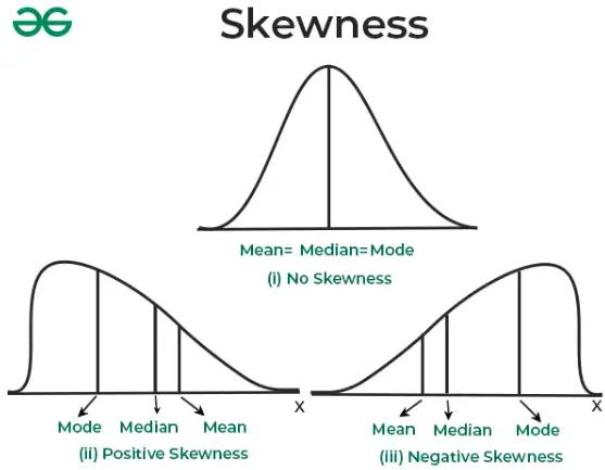
Source: Geeks For Geeks
Robust Mean and Standard Deviation Method
Robust Mean = Q2 [the median]
Note: Q2 (Quartile 2) is the middle data point if the sample size is odd. If the sample size is an even number, Q2 is the average of the two middle data points.
Robust Sigma = (Q3 – Q1) / 1.35
Note: The 1.35 number is inexact for sample sizes less than 20. Q1 is the point 1/4 of the way through the ranked data and Q3 is the point 3/4 the way through the ranked data.
yieldWerx detects and calculates PAT limits for single node and multinodal data distributions that exhibit either Gaussian, Uniform, Weibull, ChiSquare or Log-Normal signatures.
By accurately determining the distribution type, it enhances precision in failure detection, striking a balance between avoiding unnecessary yield loss and ensuring high reliability with zero defects.
PAT for Non-Gaussian Distribution
Non-normal distributions are asymmetrical, with unevenly spread data where the mean, median, and mode differ. In these cases, using the mean and standard deviation can misrepresent the data, as outliers may heavily skew these metrics.
Instead, engineers turn to other special measures to set realistic PAT limits. This approach captures outliers accurately without assuming symmetry, and it accommodates the natural skew often present in non-normal data. However, AEC recommends employing such methods with caution and detailed justification.
Below we share the basics of some of these outlier detection techniques that are equally usable in several other industries like fraud prevention, health sciences, and environment protection. In real-life scenarios, PAT calculations are much more complex and use proprietary algorithms and a combination of advanced statistical techniques outside the scope of our discussion for now.
Median Absolute Deviation (MAD)
The Mean Absolute Deviation (MAD) is the average of the absolute deviations from a central measure, typically the mean or median. You can calculate it by dividing the sum of all absolute deviations from this central measure by the total number of observations:
MAD = (Σ |Deviation from Central Measure|) / (Total Number of Observations)
MAD is a robust statistical method often used for outlier detection. It measures how much individual data points deviate from the median of a dataset, making it more resistant to the influence of outliers compared to other simple methods like standard deviation.
Interquartile Range (IQR)
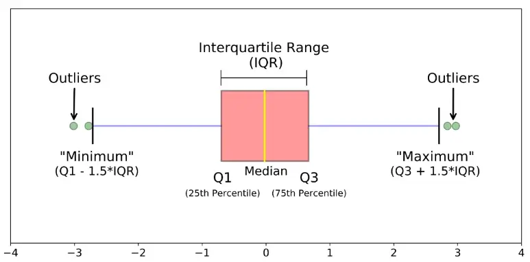
Source: DataSkill Academy
The interquartile range is a measure of spread. It tells you how data is dispersed around a central point (usually the mean).
Steps to find outliers using IQRs:
- Find the first quartile (Q1), which is the 25th percentile, and the third quartile (Q3), which is the 75th percentile.
- IQR = Q3−Q1
- Define thresholds for outliers using Q1 – k * IQR for the lower bound and Q3 + k * IQR for the upper bound, where k is typically set to 1.5 or 2 based on desired sensitivity.
For example, if k = 1.5, then:
Lower Bound = Q1 − 1.5 × IQR
Upper Bound = Q3 + 1.5 × IQR
Any data point that falls below the lower boundary or above the upper boundary is flagged as an outlier. This method might remove essential data points. So be careful while removing them.
Another related and widely used method is the semi-interquartile range (SIQR) in which IQR is divided by 2.
Adjusted Boxplot
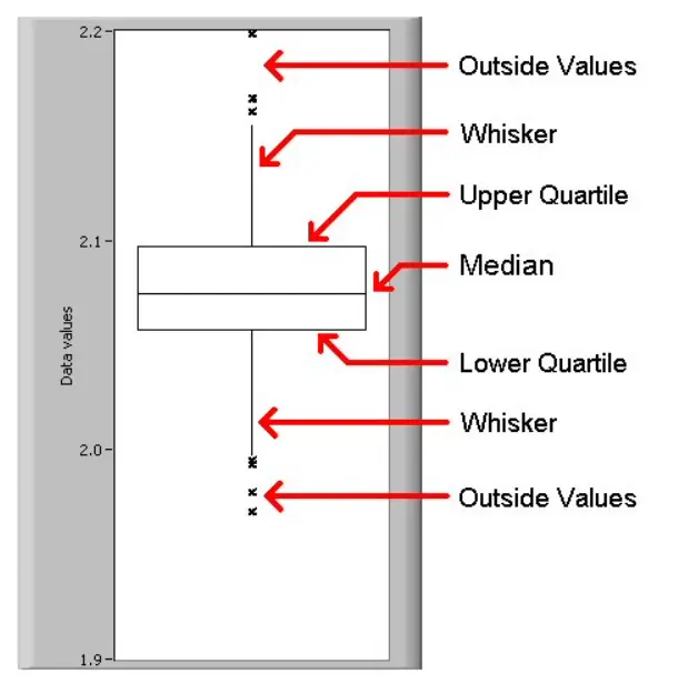
The adjusted boxplot method is known for its greater robustness in removing outliers compared to SIQR boxplot, especially in scenarios where the distribution is highly skewed in large datasets.
The adjusted box plot modifies the traditional outlier boundaries by incorporating the medcouple to scale the boundaries based on the skewness:
Upper Bound: Q3 + (1.5 × e ^ (3 × MC) × IQR)
Lower Bound: Q1 − (1.5 × e ^ (3 × MC) × IQR)
MedCouple (MC) is a robust, non-parametric measure of skewness specifically designed for use with skewed data. Unlike traditional skewness measures, the MedCouple is resistant to outliers, making it ideal for distributions with heavy tails or irregularities.
Tukey’s Method
Tukey’s Fences is a method for detecting outliers in data by defining bounds around the central 50% of the data (the interquartile range, or IQR). This method, developed by statistician John Tukey, is robust and effective for identifying outliers in both normal and non-normal distributions because it focuses on the spread around the median and IQR, making it less sensitive to extreme values.
Lower Fence: Q1 − k × IQR
Upper Fence: Q3 + k × IQR
Here, k is a multiplier that determines how far from the quartiles an observation needs to be to be considered an outlier. The most common values for k are:
- 1.5 (standard Tukey’s fences): Flags mild outliers.
- 3.0: Flags extreme outliers.
However, Tukey’s Method is suitable for symmetric or moderately skewed data. In contrast, the Adjusted Box Plot is specifically designed for skewed distributions; it modifies the outlier boundaries based on the MedCouple (MC), a robust measure of skewness.
Univariate Vs. Multi-variate PAT Analysis
As complexity in semiconductor manufacturing increases, so does the need for more advanced analysis techniques. Some types of failure categories are challenging to identify using only univariate (single variable) methods.
For example, small, distributed changes across several variables may emerge due to gradual degradation or failures due to interdependence among variables that conceal the root cause when analyzed individually.
In these cases, multivariate PAT analysis becomes essential, allowing engineers to analyze multiple parameters simultaneously. This uncovers subtle defect patterns that single-parameter methods might miss. However, selecting the right parameter combinations can be challenging, given the vast number of possibilities.
To support engineers in identifying meaningful combinations, yield management systems like yieldWerx enable simulations of multivariate relationships, often starting with two-dimensional analyses as a foundation.
Here, we discuss one commonly used multivariate outlier detection method for Automotive Part Average Testing and many other industries.
Mahalanobis Distance
The formula to compute Mahalanobis distance is:
D2 = (x-m)T. C-1 . (x-m)
where
D2 = square of the Mahalanobis distance,
x = vector of the observation (row in a dataset),
m = vector of mean values of independent variables (mean of each column), and
C = covariance matrix of independent variables
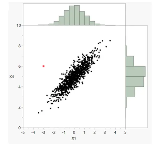
1,000 data points in two dimensions, outlier marked in red Source JMP.com
The scatterplot in the figure above allows us to visually determine outliers in two dimensions, even when the outlier is not evident from the univariate histogram distributions.
yieldWerx Zonal PAT
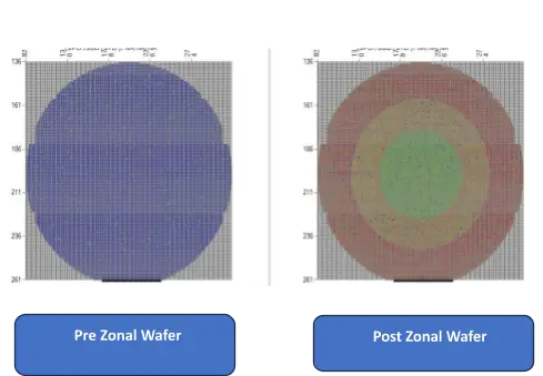
Conventional PAT detects outliers by analyzing the overall wafer population. However, dies that exhibit variations within specific zones—often caused by fab process uniformity issues—may not be detected, even if they fall within the broader distribution range.
yieldWerx enables the application of Zonal PAT, allowing users to define and configure specific zones on the wafer and categorize bin failures by zone. This capability facilitates detailed “What-If” analysis within each zone.
By analyzing variability within zones, manufacturers can identify process-specific problems. Localized detection of process drift enables targeted corrective actions, ensuring tighter control over manufacturing quality and improving overall yield.
Key Features of the YieldWerx PAT Module For Outlier Detection
yieldWerx PAT module meets all the AEC standards and comes with the following powerful features, so you don’t have to worry about setting up Part Average Testing in-house.
- You get instantaneous notifications and insights when potential outliers or anomalies are identified during the testing phase.
- Easily merge the PAT module with yieldWerx’s core application, MES/Shop-floor control systems, or automated test equipment systems like Advantest, Teradyne, and more.
- Empower your team with the ability to create and apply custom rules in PAT, offering adaptability to diverse testing and production scenarios.
- Examine past test data, spatial defect patterns, reticle failures, and more, to compare against current batches, ensuring continuous quality improvement.
- Ability to remove known Good Die where the maximum number of touchdowns has been exceeded to meet AEC guidelines.
- You can generate sophisticated reports at the touch of a button and can share reports with the team irrespective of their location.
- Utilize sophisticated techniques like GDBN and Zonal PAT to ensure reliable device shipment and minimal post-manufacture issues.
- Regular software quality checks and feature updates under the leadership of top semiconductor industry experts.
Key Takeaway
For many automotive companies outsourcing PAT to specialized providers offers distinct advantages over in-house implementation. By entrusting PAT to experts, companies gain access to state-of-the-art technology, consistent updates to testing protocols, and a team with a dedicated focus on yield optimization.
The yieldWerx PAT module, with its integration options and advanced features, enables semiconductor manufacturers to implement robust quality control without the need for extensive internal resources. This comprehensive approach to outlier detection bolsters a brand’s reputation by delivering defect-free devices.
Want to see PAT in action? Schedule a Demo to learn more about your outsourcing options and our customized testing solutions.
FAQs
What is a latent defect?
A latent defect is a faulty chip that is not immediately detectable through standard inspection or testing methods. These defects often emerge in the later part of the product lifecycle due to prolonged use or certain environmental conditions.
What is the difference between an outlier and an anomaly?
Anomalies are unexplainable values deviating too much from the base distribution. For example, in a dataset containing the age of students in a college, the value of -10 is an anomaly, as age cannot be a negative number.
Outliers are unlikely events or data points significantly different from points in a dataset. For example, in the same college dataset, the student’s age could be 97, i.e., an older person.
In our case, an outlier is a chip that has passed the original manufacturing tests but differs from the lot while showing abnormal characteristics and is more likely to fail in the field.
How does PAT differ from traditional binning?
Traditional binning categorizes parts as pass/fail based on test limits. PAT uses statistical methods to detect anomalous parts based on average performance rather than fixed limits, making it more sensitive to deviations within a production batch.
How is the PAT test performed?
During the Electrical Wafer Sort (EWS) phase, unpackaged ICs undergo testing. This involves a mechanical probe making contact with each IC’s pads on the wafer, where a probe card connects to the test equipment through cables. An automated system then performs sequential testing on each die across the wafer.
Throughout this testing, a datalog file records measurement results to compute the mean (μ) and standard deviation (σ). With these values established, outlier parts that passed the test but fall outside the acceptable range can be accurately identified.
At what stage PAT testing is performed?
You can implement it at the wafer or final test stage or both. However, by identifying anomalies at an early stage, engineers can implement corrective actions before defective components are made and scrapped.
What is the difference between PAT and GDBN?
PAT methodology separates chips that are different from other chips, which have been normally produced, GDBN identifies a working die surrounded by a failing die and removes it from the lot as a precaution.
How does PAT help improve yield?
PAT enhances overall yield quality and reliability by identifying and removing outliers that may still technically pass test limits but show abnormal behavior.
What are some typical PAT Electrical Tests recommended by AEC?
AEC – Q001 guidelines Rev-D states some of these tests:
- Pin Leakage Test
- Standby Power Supply Current (IDD or ICC)
- IDDQ testing
- Over-Voltage Stress Test
- Output Response Time
- Output breakdown voltage
- Output leakage
- Output current drive
- Output voltage levels
- Low/High temperature
Are there any limitations of the traditional PAT test?
Legacy solutions for part average testing rely heavily on electrical testing only. Advances in wafer scan technology promise additional capabilities.
References

